How to integrate a Neural Network in your SBC

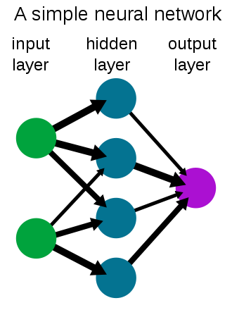
In this article we will learn how to integrate a neural network in the SBC. We will create a 3-layer neural network to approximate the function sin(x).

The process is divided into two parts: 1. training the network, which will be done on the PC and; 2. running the network, which will be done in the SBC.

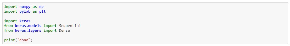
For this part we will use Jupyter notebooks, with the Keras, Numpy and Pylab libraries.

Step 1. Import necessary libraries

Step 2. Create the training dataset

Our dataset consists of 10000 random numbers in the range 0 – 2*pi as input X and their corresponding sin function as input Y. Note that we have adjusted the range of Y to range from 0 to 1.

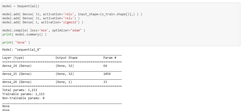
Step 3. Create the neural network

To create the neural network, we create a model object and add 3 layers to it. This is done through the API provided by the Keras library.

The number of neurons will be 32 for the first layer, 32 for the middle layer, and 1 for the output.

We will use the relu and sigmoid activations.

The optimizer used is Adam and the error function MSE.

The number of network parameters is 1153.

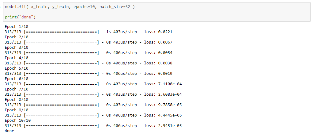
Step 4. Training

When training, the neural network uses the dataset to adjust its parameters in such a way that the error is minimized.

In this case, we passed the entire dataset through the network 10 times, in 32-sample batches.

As we can see, at the end of the training, the error is very small, 2.5e-5.

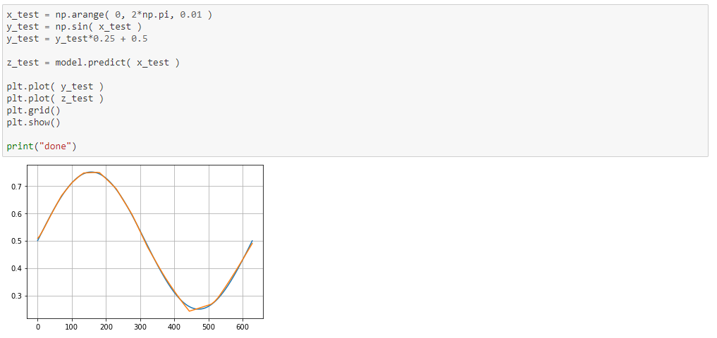
Step 5. Verification

Now we will test the neural network one last time and compare it to the expected values. As seen in the graph, the network approximates the sine function quite well.

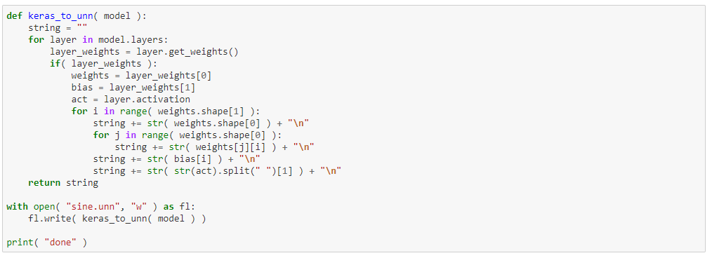
Step 6. Export the data

This function allows you to export the weights of the neural network to a text file and then load it from the SBC.

Part 2. Execution on the SBC

First of all, we will review the implementation of the neural network.

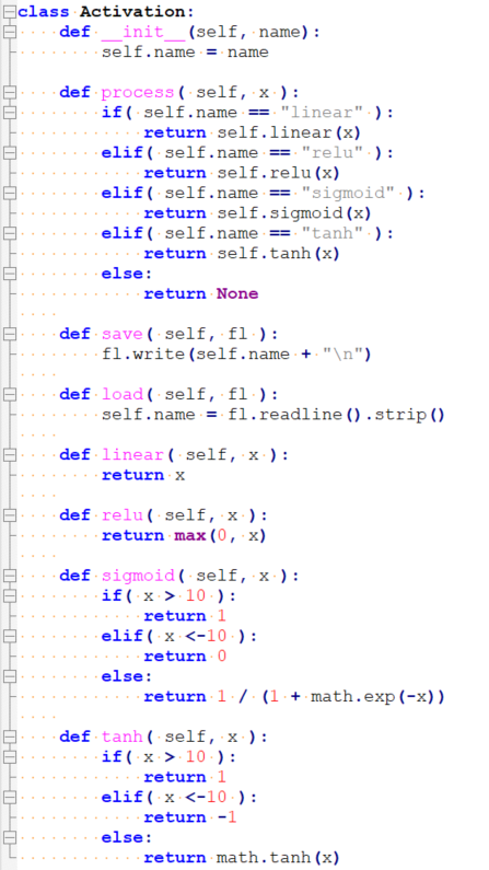
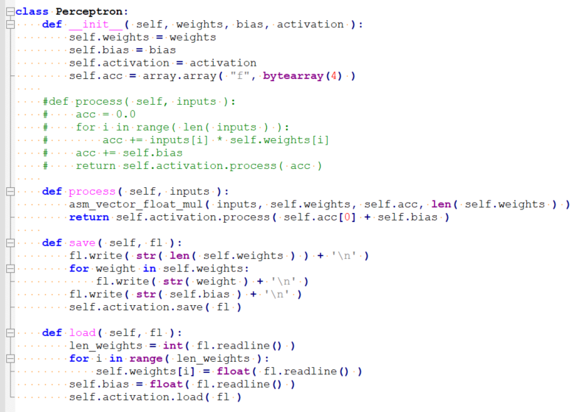
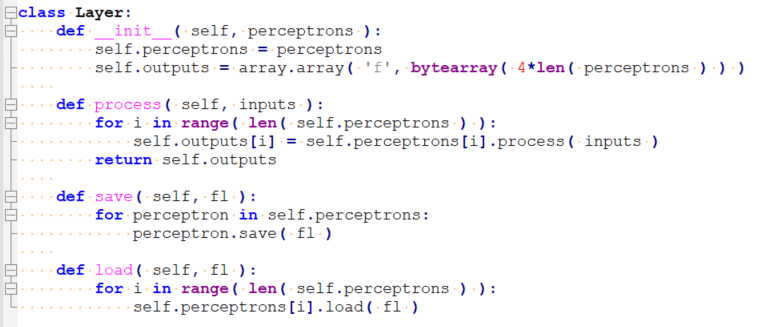
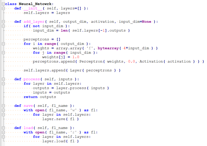
The neural network is divided into 4 classes: Neural_Network, Layer, Perceptron and Activation.

Each class basically has 1 method called process that is in charge of doing all the work, as well as loading and saving methods.

The Activation class, implements the linear, relu, sigmoid, and tanh activation functions.

The Perceptron class is responsible for performing all multiplications. Note that the vector multiplication function is implemented in ASM so as not to sacrifice performance.

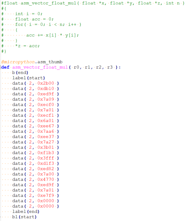
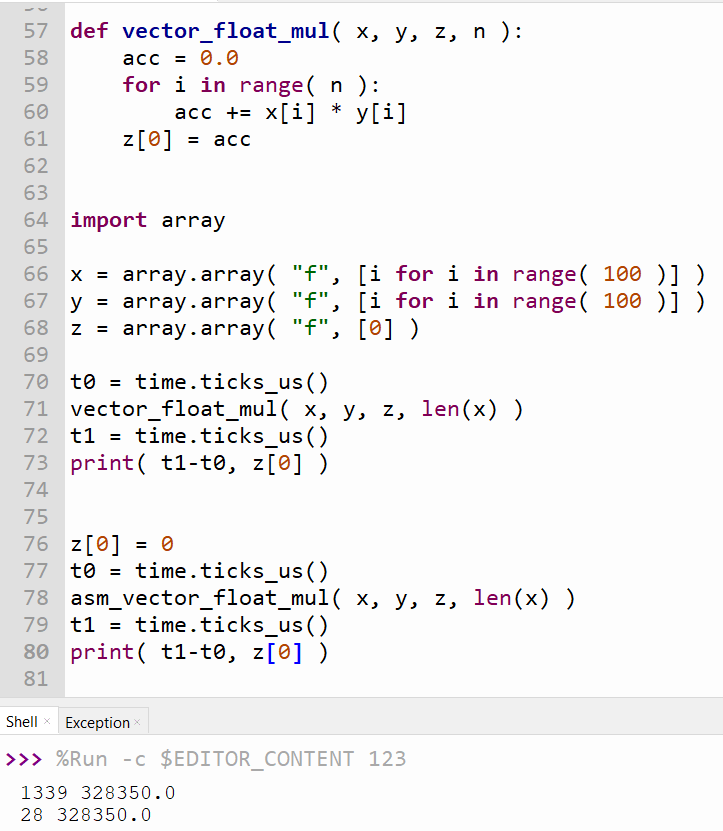
ASM vs Python implementation

The vector multiplication is responsible for the most part of the CPU usage, so implementing it on ASM allows improving the library performance by a lot. In this example, a simple 100×100 vector multiplication is performed. A python implementation takes 1339 us, meanwhile, the ASM implementation only takes 28us. This is about 50x faster while preserving the same output values.

The Layer class groups a few perceptrons in parallel.

The class Neural Network stacks all the network layers.

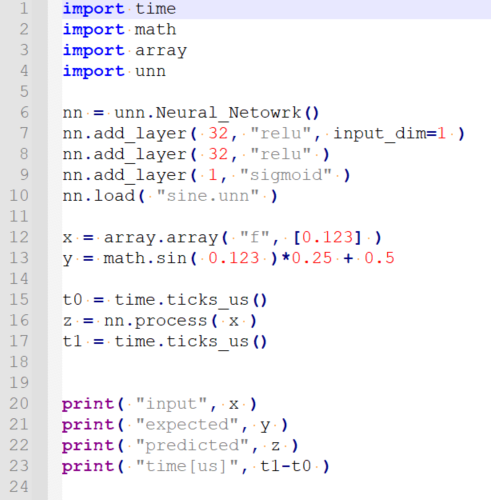
Finally, we can review/check the use of the network.

We will copy the file with the weights to the SBC and execute the following main.py.

This code loads the network from the sine.unn file and calculates the sine of 0.123 and then displays the value obtained by the network and the real sine, as well as the calculation time in microseconds.

Output:

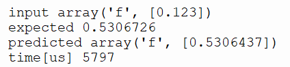
As we see, the output approximates the expected value with 4 decimals.

This network, with 1153 weights, required 4612(1153*4) bytes of RAM to store weights in float value and 5.8ms to process.